English PDF · LaTeX / Tavotto sources and data · Portable task query · Task metrics CSV
Can an agent take a terminal model and two loading steps, inspect the model, allocate computing resources, complete a solve, and return verifiable curves and contour plots? This project connects HyperMesh, Abaqus, and ParaView through three MCP services. All three independent sessions completed a real terminal contact case. The session with MCP tools and engineering procedures took 21.82 minutes and produced 108 frames, with a peak actuator force of approximately 1.434141 N.
Start with a loading request
CAE automation often begins with a script: import a model, define sets, submit a job, and extract results. Agents make script generation easier, but many engineering difficulties lie between these operations. Which region does “the right end” identify? Does an application process exiting mean the solve succeeded? Can an extrapolated nodal stress be compared directly with integration-point stress? What changed after a failure, and which output should the next operation read?
This project makes those questions part of the tool interface. The agent interprets the goal and selects actions. Tools validate inputs, execute native applications, retain logs, and return actual artifacts. The focus is execution reliability and traceability. The engineering measurements described here were collected on October 12, 2026.
The terminal task retains the existing materials, sections, and mesh. The male roots and shield root are fixed. The plate first moves along global , then moves with the female terminal by along global . The friction coefficient is 0.13. Regions, directions, and sets were confirmed before execution. For new ambiguous descriptions such as “left” or “down,” the agent presents candidate regions and a coordinate interpretation before changing the loading conditions.
Three MCP services and 54 tools
MCP is the protocol through which an agent calls tools. The project separates the native applications into three services with a shared execution layer: HyperMesh for geometry and mesh, Abaqus for models, solving, and ODB access, and ParaView for result inspection and visualization.
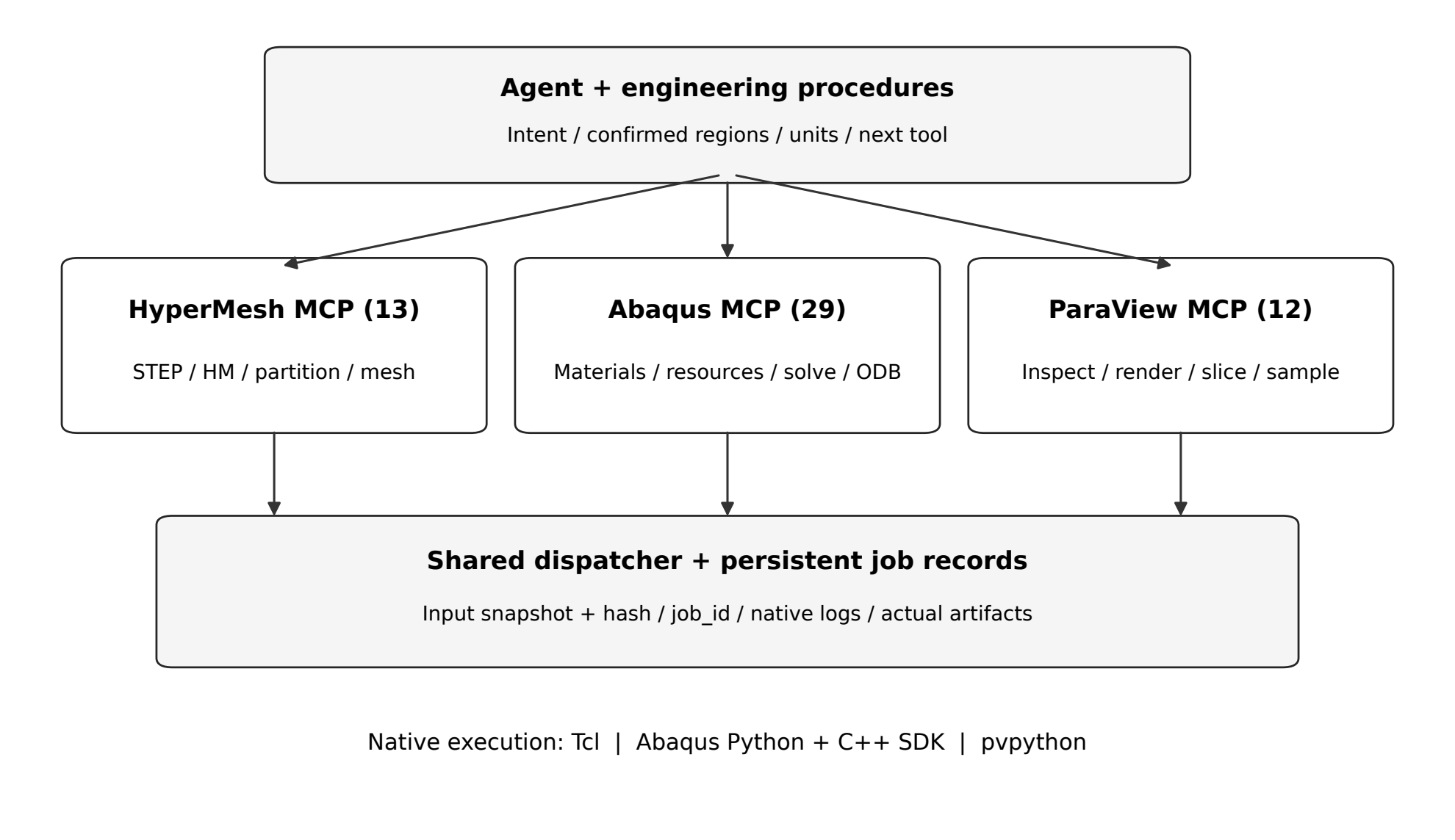
| Service | Tools | Capabilities |
|---|---|---|
| HyperMesh | 13 | STEP import, HM inspection, partitioning, tetrahedral mesh, INP export, Tcl. |
| Abaqus | 29 | Materials, regions, loading, resources, solve, diagnosis, repair, ODB conversion. |
| ParaView | 12 | Array/frame inspection, rendering, slices, line sampling, images, Python. |
Each service includes six common management tools: capabilities, job status, job listing, artifacts, logs, and cancellation. The total of 54 includes these application-specific management interfaces; it does not represent 54 separate analysis algorithms. The full catalog is included in the article source archive.
Scripts execute in the appropriate application runtime: Tcl in HyperMesh 2017, Python or the C++ SDK in Abaqus 2025, and pvpython in ParaView 6.1. The general Python service handles protocol, scheduling, and input checks instead of mixing proprietary binary APIs and interpreters.
Three services retain the distinct input contracts, runtimes, and failure modes of preprocessing, solving, and postprocessing. Resource management belongs to the Abaqus service so different services do not independently reserve the same solver budget. The ODB2VTK executable also works directly without MCP.
Long tasks need persistent state and real files
A tool accepts a long operation and returns a job_id. An independent background dispatcher manages execution while the client polls persistent state. Only succeeded permits passing the returned artifact paths downstream. Neither queued nor running means completion.
Each job retains its request, settings snapshot, native script, logs, state, and result index. INP dependencies are copied recursively through INCLUDE files and recorded with SHA256 hashes. Resource plans bind to the same input closure. If inputs change while a job waits, the old plan cannot silently authorize the new files. Sources remain read-only, and repairs produce new inputs.
A complete Abaqus success check requires the native completion marker, both steps reaching their prescribed endpoints, and a nonempty, closed, newly generated ODB. An existing ODB or one converged increment is insufficient. ParaView then checks actual arrays, frame counts, and ranges rather than returning an image as the only evidence.
An independent dispatcher also addresses process lifetime on Windows, where closing a client can terminate descendant processes. Accepted solves should survive an individual tool connection. This is local execution management, not a replacement for an operating system or cluster scheduler.
An independent C++ ODB converter
ODB2VTK uses the official Abaqus C++ ODB API and its bulkDataBlocks() interface for contiguous field reads. It avoids accessing each FieldValue object separately. Mesh data, label mappings, and section assignments are built once and reused across frames. Binary VTU files store results, and a PVD file indexes the selected frames.
The CLI offers inspect, menu, and convert. When options are omitted, it detects the last step containing frames, its final frame, all nonempty instances, and available U and S:MISES. Explicit options select multiple steps, frame lists or ranges, section points, output position, deformation scale, and real or imaginary complex components.
.\native\odb2vtk\odb2vtk.cmd inspect --odb "input.odb"
.\native\odb2vtk\odb2vtk.cmd menu --odb "input.odb"
.\native\odb2vtk\odb2vtk.cmd convert --odb "input.odb" --step all --frames all --fields "U,S:MISES" --avg 75 --regions section --output "exports\terminal"
Exports include per-frame VTU files, collection.pvd, and manifest.json. ODB access is read-only. Missing values remain NaN, unsupported elements fail by default, and older ODBs are not silently upgraded. The Windows launcher sets the Abaqus DLL search path for its process; another machine still requires compatible native runtime libraries.
Avg 75 depends on regions and operation order
Following the Abaqus/CAE default region definition, averaging regions follow actual section assignments. Matching material or section names do not merge two assignments. Elements without an assignment are isolated and reported rather than assigned an invented common region.
For a scalar such as Mises stress, the converter extrapolates the tensor to element nodes, computes the scalar, and then applies the region and threshold test. Relative variation at a node is The numerator uses contributions at that node; the denominator uses the range of all valid extrapolated contributions in the current averaging region. For a nondegenerate region, permits an equal-weight average. Equality with the threshold retains discontinuities. If the regional range is zero and contributions are identical, a positive threshold permits averaging. A threshold of 0 or off disables it.
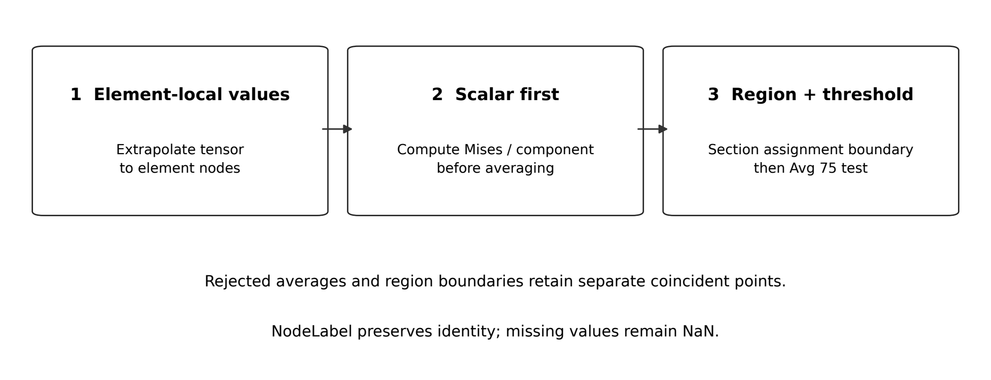
Arrays expose S_MISES_Avg, variation percentage, whether averaging was actually applied, and SectionAssignmentId. No subsequent Clean/Merge Points or Cell Data to Point Data operation is inserted: either could erase the discontinuities deliberately preserved by the export.
This implements scalar-before-average within section assignments. It does not reproduce additional shell/membrane feature-edge boundaries or tensor-after-average modes. Stored integration-point and extrapolated nodal values must also remain distinct: the final-frame maximum integration-point Mises is approximately 644.00 MPa, while the Avg 75 extrapolated nodal display reaches approximately 1355.07 MPa. These are different output locations.
Choosing computing resources automatically
The resource tool scans INP files, INCLUDE dependencies, and assembly instances for node counts, element types, procedures, contact, and NLGEOM. Repeated instances contribute their actual assembly multiplicity. For this solid mesh, is a sizing proxy for degrees of freedom. A factor of 1.5 accounts for the presence of contact, producing a weighted size . This is not the solver’s equation count after constraint elimination.
The initial CPU tier is Physical cores, project budgets, user limits, and any configured license allowance further constrain the result. Memory caps start at 15%, 30%, or 50%, then respect available memory and shared budgets. abaqus_plan_resources creates the plan; abaqus_submit_job consumes it and revalidates the inputs at startup.
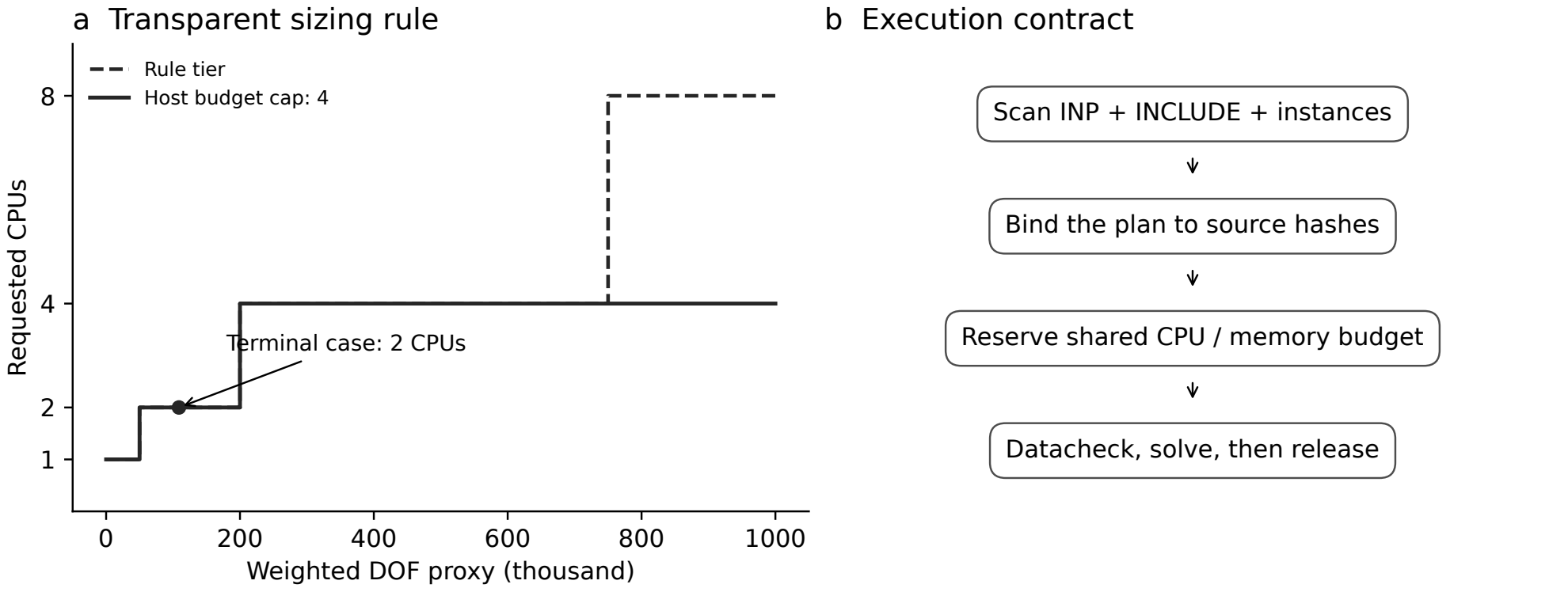
This case uses 2 CPUs and a 15% memory cap. All comparison groups received the same caps and pure-thread configuration so resource differences would not be confused with tool differences. Shared reservations constrain the aggregate CPU and memory budgets of solves started by these tools. Jobs wait when the budget is unavailable and release reservations after completion.
These are transparent initial sizing rules, not calibrated optimal configurations from repeated multi-scale CPU sweeps. Under the Abaqus execution parameter definitions, Standard memory is an allocation cap; the same interpretation does not cap the actual Explicit analysis phase. The service does not control externally launched solves or claim that a configured license limit is a live license-pool query.
Read failure evidence before generating a repair
abaqus_diagnose_job reads actual .dat, .msg, .sta, and log files. It returns bounded original context, file hashes, classifications, and eligible repairs. Unknown failures remain unknown rather than receiving a guessed universal fix.
The automatic scope of abaqus_repair_job is deliberately narrow. Evidence-supported changes can reduce the initial static increment or raise the maximum increment count. A new INP, diff, and change record are retained before replanning and datacheck. Total loading, materials, friction, fixed regions, and total step duration are preserved. Physical-condition changes require explicit confirmation.
The product session’s first datacheck actually found an empty node-based surface definition. Using native diagnostics, the agent established that the surface was unused, commented out that definition and removed a blank line through an advanced script, retained the diff, and then passed datacheck and solved. This demonstrates diagnostic tools working with native scripting; it does not mean the restricted numerical repair tool handles every syntax failure.
Material and section records, and the role of a Skill
Existing definitions may come from INP, CAE, or HyperMesh models. Library tools stage a preview before committing imports and retain original keywords, declared units, provenance, and revisions. Updates require expected_revision; sections reference a specific material revision. Export binds definitions to an explicit ELSET, and units are never silently converted.
The tetrahedral loading template supports homogeneous solid sections within its stated scope. Composite sections, unknown keywords, and unresolved orientation definitions are rejected or reported. The terminal model keeps its original materials and sections, with no invented demonstration elasticity.
A Skill supplies orchestration procedures: check units and sets, confirm ambiguous spatial descriptions, wait for long tasks to succeed, consume real artifacts, preserve averaging boundaries, interpret native warnings, and retain failed attempts. Deterministic validation stays in MCP tools. The product group enabled both MCP and engineering procedures; the comparison does not isolate the Skill’s contribution.
The terminal case: preprocessing through postprocessing
Inputs are an already-meshed single-pair terminal INP and an HM companion extracted from a larger assembly. The model contains one female terminal, two male blades, a shield, and a prepress plate. The INP is authoritative for labels, materials, sections, and eight contact pairs. HM supports native model inspection; its node labels do not replace INP labels.
The model has 11,240 C3D10M elements. Each male-root set contains 21 nodes, and the shield-root set contains 159, for 201 fixed root nodes. A 72-node region controls the female through an RP. The plate node surface has 1061 nodes and couples to a separate RP.
| Setting | Definition |
|---|---|
| Prepress | Plate mm, ; female remains stationary. |
| Insertion | Retain plate ; plate and female simultaneously reach mm. |
| Contact | Friction 0.13, hard contact, finite sliding, NLGEOM=YES. |
| Static controls | Initial increment 0.01, duration 1, minimum , maximum 0.05, 10000 increments. |
| Other constraints | Fix RP rotations and non-driven translations; fix male/shield root translations. |
The execution sequence is native HM inspection, INP mesh and region checks, preparation of two new loading steps, a resource plan, datacheck, evidence-based error handling, and a complete solve. The agent then reads control-point histories, energies, and original integration-point results from the new ODB, converts all steps and frames, and checks and renders the data in ParaView.
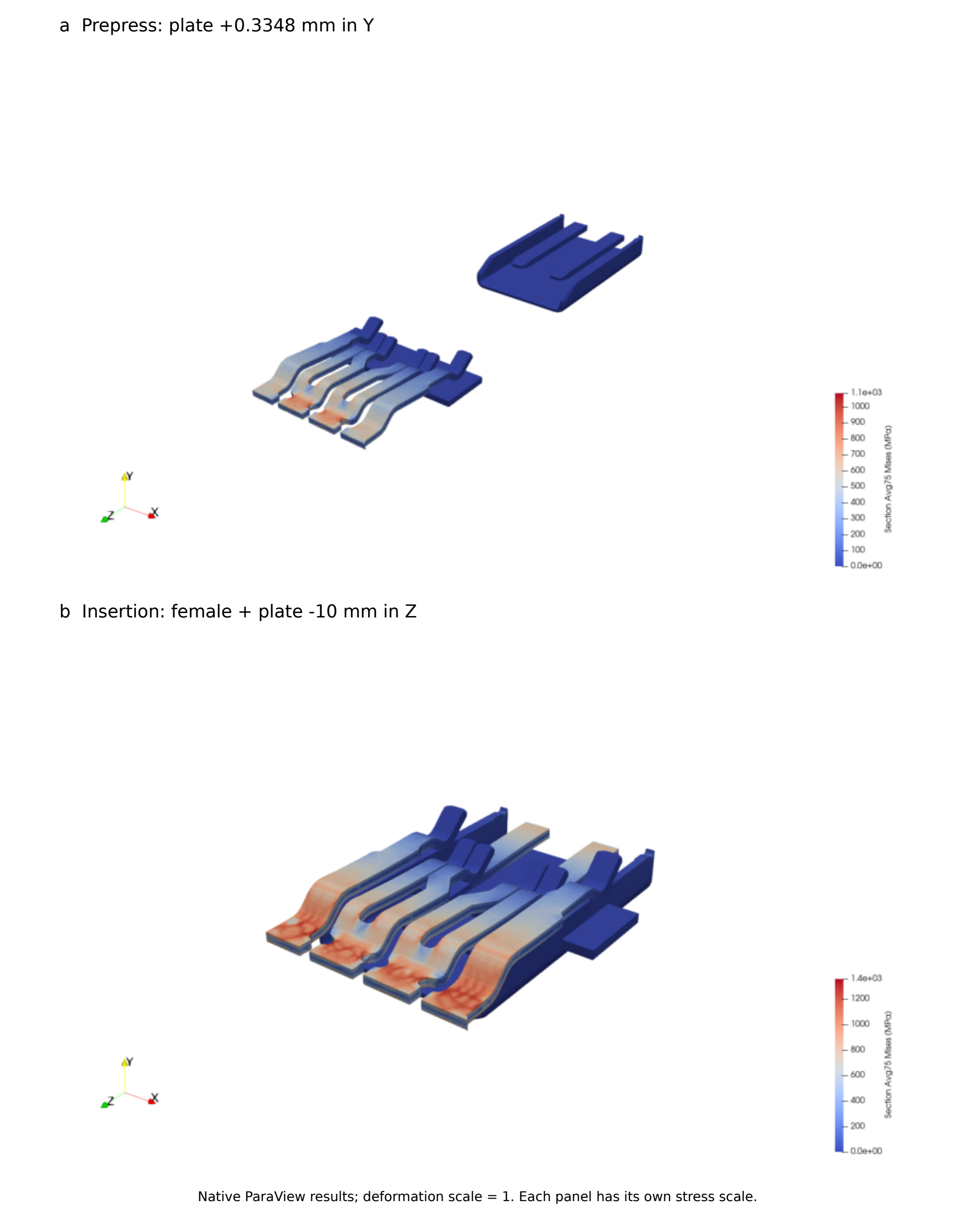
This case retains the existing mesh. Preprocessing covers model and region checks, coupling, and loading preparation. STEP import, partitioning, and tetrahedral meshing are implemented tools, but this experiment does not start with automatic CAD remeshing and reconstruction of every contact definition. The two steps cover prepress and insertion, with no added withdrawal step.
Define results numerically
Insertion force combines the two moving RPs’ global reactions and projects them onto the insertion direction: This avoids adding internal forces from both sides of contact. The new product ODB contains 25 Prepress frames and 83 Insertion frames, totaling 108. Both steps reach their endpoints, and stored control displacements match the specified values.
| Metric | Value |
|---|---|
| Final prepress plate (mm) | 0.334800005 |
| Final insertion female / plate (mm) | |
| Peak actuator force (N) | 1.434141 |
| Final actuator force (N) | 0.974671 |
| Final maximum integration-point Mises (MPa) | 644.000061 |
| Final maximum PEEQ | 0.009152083 |
| Maximum absolute final stored RF component sum (N) |
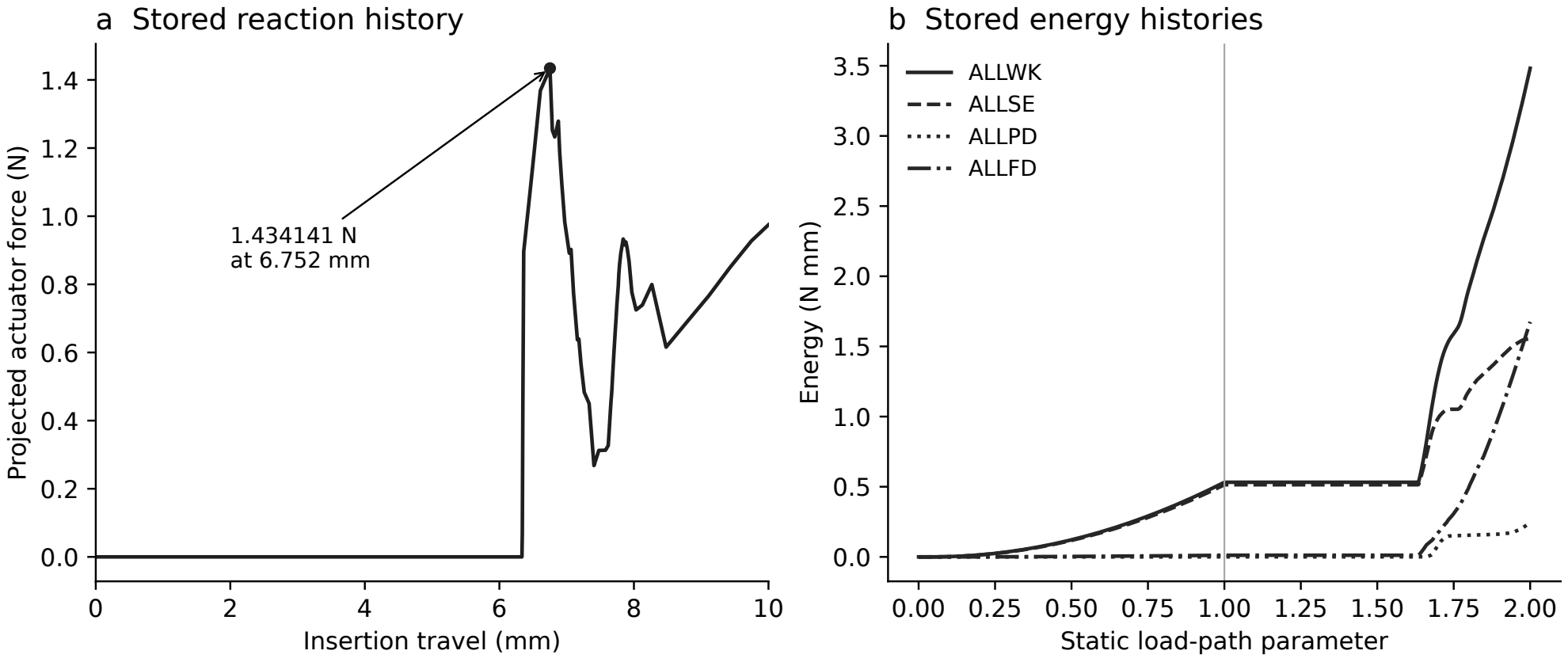
Selected final energies are approximately ALLWK 3.4821 Nmm, ALLSE 1.5564 Nmm, ALLPD 0.2456 Nmm, and ALLFD 1.6753 Nmm. The visible remainder after subtracting the latter three from external work is approximately 0.138% of ALLWK. This checks only these stored quantities, not every solver energy term.
PVD uses sequential indices 0–107 because step-boundary time values can repeat. Original step names, frame values, and physical total time remain in the manifest and data. Sequence index 107 is not 107 seconds. If exported coordinates already include displacement, ParaView does not apply a second Warp.
Three independent sessions: all completed, with different paths
All groups received the same inputs, engineering request, and resource caps. Each had to produce a new ODB and could read vendor documentation, write scripts, and use the same standalone C++ converter. Groups could not share scripts, historical solutions, or results. Solves ran serially, without an imposed overall time limit.
| Group | Tools | Distinguishing conditions |
|---|---|---|
| A | Three CAE MCPs and procedures | Requires actual MCP calls and a new solve. |
| B | Native file and terminal tools | Writes native scripts; no CAE MCP; used generic planning procedures. |
| C | Native file and terminal tools | Different model and host; not a single-factor comparison. |
An independent evaluator reopens every new ODB to read displacements, reactions, energies, and integration-point results, and checks native success markers, mesh data, VTK files, and images. The 100-point artifact checklist assigns 5 for input preservation, 10 for model-definition preservation, 25 for a complete new solve, 15 for control displacements, 10 for reaction/energy checks, 10 for native preprocessing, 10 for 108 frames and regional averaging, 5 for images and curves, and 10 for resource records and datacheck. It is neither a general success rate nor a design-validation score.
| Group | Checklist | Minutes | Tool calls | MCP calls | Peak (N) |
|---|---|---|---|---|---|
| A | 100/100 | 21.82 | 109 | 47 | 1.434141 |
| B | 100/100 | 27.24 | 81 | 0 | 1.434141 |
| C | 100/100 | 56.13 | 243 | 0 | 1.434150 |
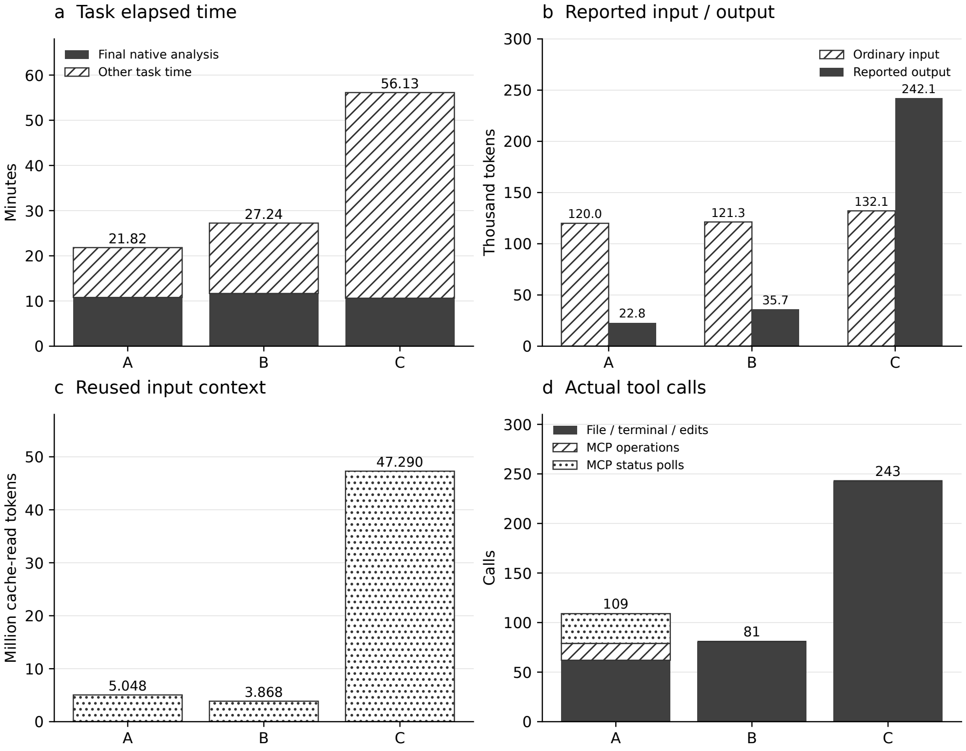
A’s client wall time was approximately 19.9% lower than B’s in this experiment. Final native analyses took 647, 700, and 637 seconds. Remaining task times were approximately 662, 935, and 2731 seconds, including preparation, checking, diagnosis, postprocessing, network operations, and waiting. They are not isolated model-inference times. Much of the observed difference lies in engineering coordination rather than solver acceleration.
| Group | Ordinary input | Cache reads | Output |
|---|---|---|---|
| A | 119970 | 5048320 | 22840 |
| B | 121289 | 3867776 | 35711 |
| C | 132141 | 47289728 | 242125 |
Repeated context across turns contributes to these totals; they are not unique query lengths. An input counter can include or exclude cache reads depending on the client, so categories are separated. Reasoning tokens already counted within output are not added again. Cross-provider tokenizers and routing counters were not independently calibrated, and these figures do not establish equivalent compute or actual billing.
The measurement window spans submission of each engineering request through task completion and client exit, using only that task client’s final usage report. Article writing, LaTeX compilation, Tavotto figures, experiment setup, independent evaluation, presentation camera work, and publication are excluded.
Failure traces explain more than one total score
A completed with structured inspection and one evidence-supported input repair. B organized native scripts and delivered the same required artifacts. C repeatedly built diagnostic inputs around contact and coupling keyword layout, then completed after CAE import and export normalized the keywords.
The groups retained 1, 1, and 15 distinct datacheck data files containing errors. These counts represent diagnostic files, not 15 failed full solves. The request limited evidence-supported failed modifications to two; native groups performed more diagnostic attempts. This process deviation remains documented and is not included in the 100-point artifact checklist.
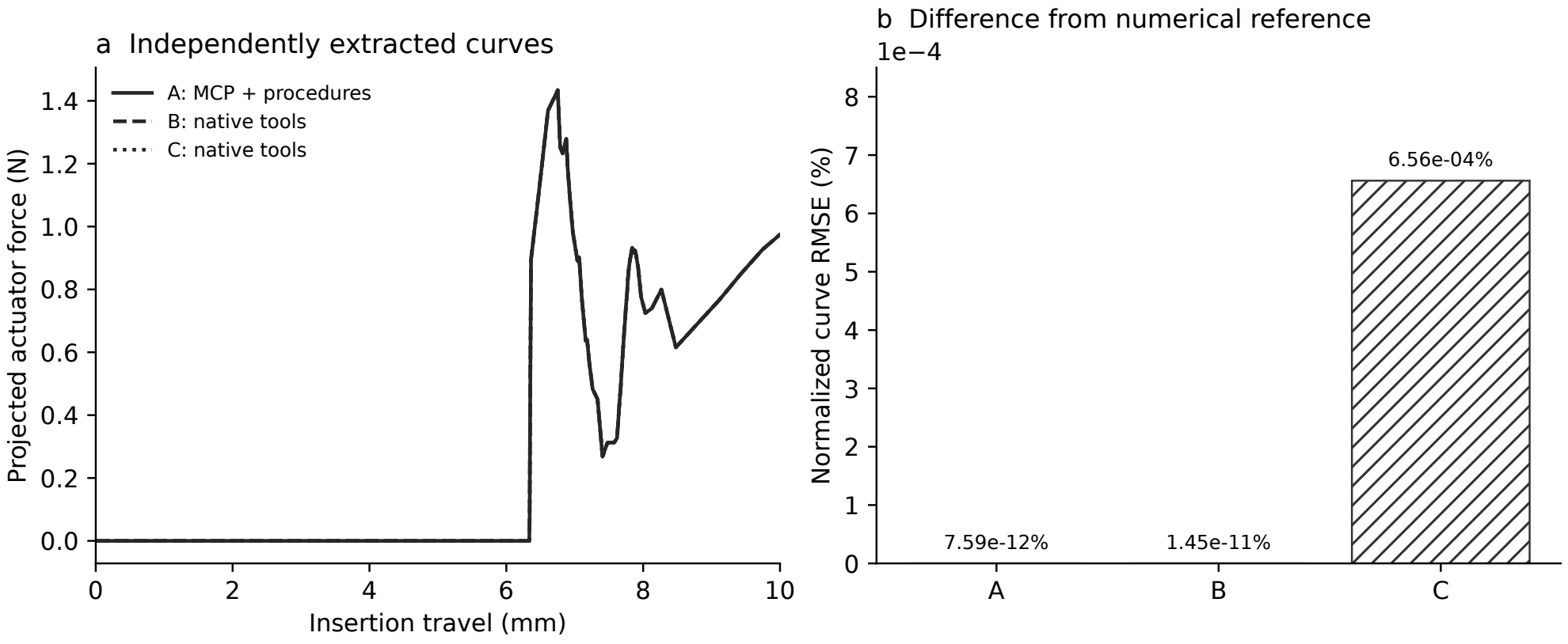
C’s peak differs from the numerical reference by approximately 0.000623%, and its normalized curve RMSE is approximately 0.000656%. All groups can complete the professional task, making execution path, context growth, and recovery behavior useful comparison targets. One case, one session per group, and simultaneous use of MCP and a Skill cannot establish a general capability ranking or isolate their causal contributions.
Engineering facts that remain after completion
The product group’s native records contain 6 dat warnings and 73 msg warnings, including 23 negative-eigenvalue warnings. They identify 618 distorted elements. C’s normalized-input inspection reports 620 distorted elements in its own context; this cannot be presented as a mesh-quality improvement.
Negative eigenvalues in nonlinear contact may accompany tangent-stiffness changes, but convergence alone cannot rule out instability or constraint problems. Distortion, material definitions, contact regions, and mesh sensitivity still affect physical credibility. This case establishes tool execution, result extraction, and traceable delivery for a specified model and confirmed conditions. It does not establish experimental correlation, lifetime performance, a complete insertion–withdrawal hysteresis loop, or industry-company endorsement.
Inputs, query, and inspectable evidence
The measured INP is 3,460,015 bytes and the HM companion is 2,313,685 bytes. Their SHA256 fingerprints are included in provenance data. Published attachments contain measured statistics, curves, a portable query, LaTeX, and editable Tavotto sources; engineering models and large solver databases are not released.
The following summarizes the portable editorial adaptation of the original task. Local absolute paths and experiment-directory isolation wording are removed, with engineering conditions preserved. The full portable query and original query fingerprint are provided with the attachments.
Inspect terminal_pair.hm and terminal_pair.inp. Retain existing mesh, materials, sections, and eight contact pairs. Fix the confirmed male and shield root sets and couple the female and plate control regions to RPs. Prepress: plate moves 0.3348 mm along global . Insertion: retain prepress while plate and female move 10 mm along global . Use friction 0.13, hard contact, finite sliding, NLGEOM, and exactly two steps. Record a resource choice capped at 2 CPUs and 15% memory, run datacheck, then submit a new solve. Read stored RP displacements and reactions, energies, and original integration-point stresses. Convert all steps and 108 frames using section-assignment Avg 75. Inspect the data in ParaView and return endpoint contours, state files, and the actuator curve. Retain native errors and input diffs without changing physics to force convergence.
Native interface references
Vendor documentation describes bulk ODB access, averaging regions, and job-execution parameters. The implementation scope is stated beside each capability.
English PDF · LaTeX / Tavotto sources and data · Portable task query · Task metrics CSV