English PDF · Chinese PDF · Bilingual LaTeX and figure sources
What this article covers. The difficulty in connector finite element analysis is not simply solving one model. It is making the same physical model generate many reliable samples and explaining when those samples lose contact performance. This article follows an engineering route through reduction, parameterization, scheduling, postprocessing, and boundary search.
Public scope. Customer, product, and loading details are anonymized. This article contains no actual models, original tolerance vectors, unpublished contact-force data, or performance figures. The sampling plot is an independently generated method demonstration; the other figures are schematic. The added coupled search has passed offline code and coordinate checks. Actual failure boundaries still require complete solves with the matching model.
Three requirements before scaling up
A usable batch simulation system must satisfy three distinct requirements: physical interpretability, numerical checks, and recoverable execution. Reducing solve time is only the first step. If samples use different contact settings, tolerance application contaminates the baseline, or a solver interruption is counted as contact failure, faster computation does not produce a credible operating boundary.
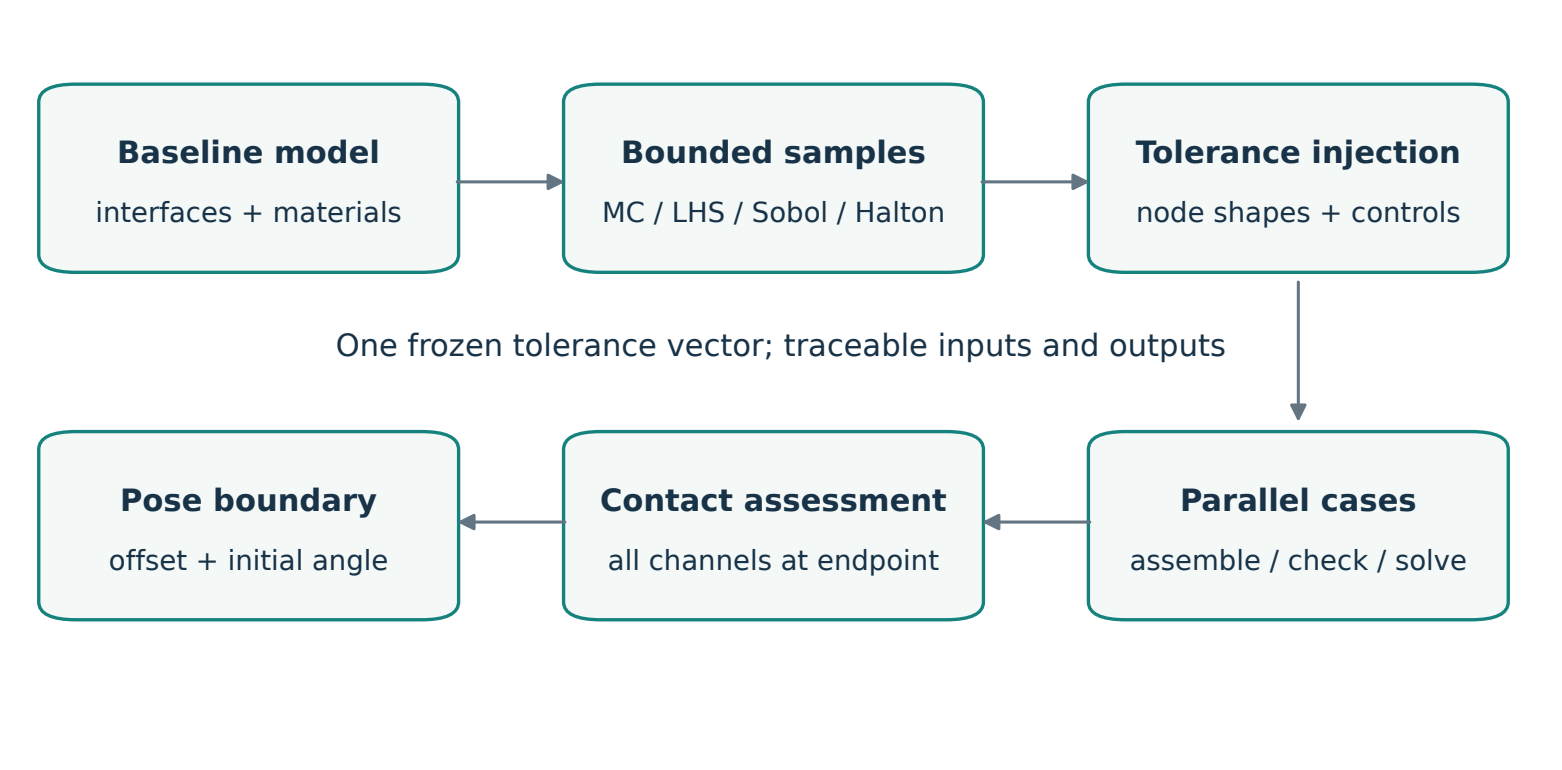
Figure 1 summarizes the route: substructures reduce repeated computation; explicit variable mappings produce samples; and consistent contact metrics connect batch statistics to pose search. Each stage retains the identity and provenance of its inputs.
The problem is a family of models
Connector mating is a nonlinear contact problem. Geometry, local stiffness, initial gaps, and the loading path jointly determine the final contact state. One analysis of nominal geometry answers a question about a single configuration. Manufacturing deviations introduce a family of responses; assembly offsets and angular misalignment add further conditioning variables.
The problem can be written as where is the manufacturing-tolerance vector, is the initial assembly pose, and contains physical settings such as materials, friction, prepress, and insertion path. The operator represents finite element modeling, assembly, and solving. Outputs include contact-force curves and endpoint metrics.
This formulation separates manufacturing tolerances, assembly pose, sampling design, and physical settings. A comparison of sampling methods holds pose and physical settings fixed. A pose-boundary search holds the same manufacturing-tolerance vector fixed. Otherwise, changes in the response cannot be attributed clearly.
The work therefore has two layers. First, deterministic analysis must be efficient enough to support batch execution. Second, the same foundation introduces tolerances and automated failure-boundary search. The focus here is the engineering connection between these layers rather than adding a separate predictive model.
Reduce the repeated work with substructures
What CORE and SUB mean
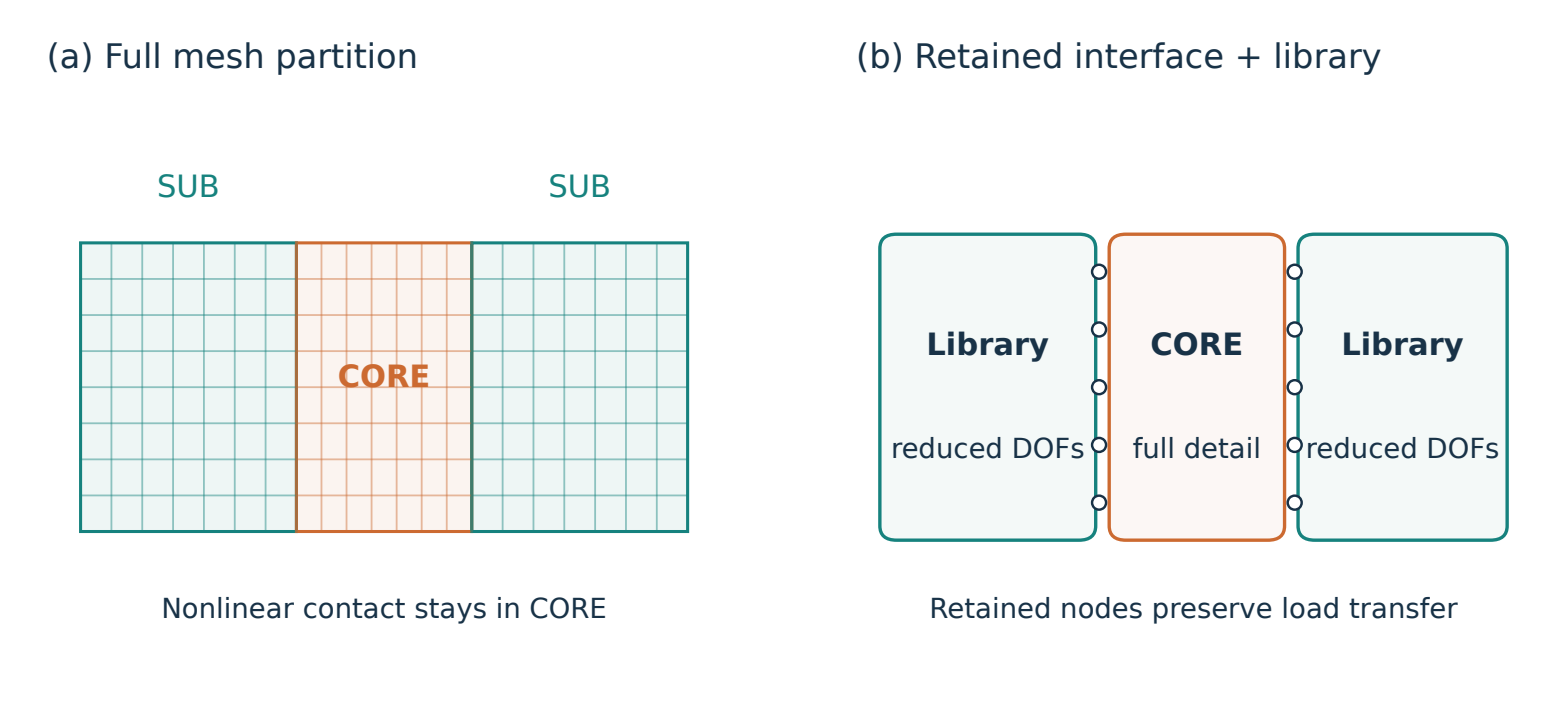
The finite element method (FEM) discretizes a continuum into nodes and elements. Here, CORE names the retained nonlinear contact region, and SUB names a region suitable for condensation. These are engineering partition names, not material types or specific solver element names.
Figure 2 illustrates the partition with an abstract mesh. Contact and local deformation remain in CORE, while the more distant structure transfers loads through retained interface nodes. Element count alone cannot determine the partition: contact might enter the reduced region, material nonlinearity may matter there, and the interface must retain the correct motion degrees of freedom.
Why static condensation reduces repeated work
Partition a linear substructure into internal degrees of freedom and retained degrees of freedom : Eliminating the internal degrees of freedom gives The inverse is mathematical notation. Implementations normally solve linear systems rather than explicitly constructing the entire inverse. Reduction happens during substructure generation; the usage stage assembles the resulting library with CORE.
The benefit comes from reuse, not deleting a region of the model. Multiple samples that change only CORE can reuse a verified library when the substructure and its interface definition remain applicable. Changes to substructure geometry, materials, retained degrees of freedom, or generation conditions invalidate that assumption, even when the filename stays the same.
Files form a consistent set
An input deck, usually .inp, records the mesh, sets, and keywords. Substructure-related .sim, .sup, and output database (ODB, .odb) files have different purposes. They cannot be replaced independently merely by matching extensions. They must originate from a compatible generation job and agree on interface labels.
Library provenance is therefore an input: generation files, retained sets, model identity, and validation results are recorded. Batch assembly creates interface sets from labels instead of guessing nearest coordinate points in a large model. Abaqus documentation [1] describes the underlying method; suitability must still be checked for the current model.
Parameterization starts with a successful GUI operation
Record the working operation, then wrap it
A correct graphical user interface (GUI) operation is a reliable starting point for automation. HyperMesh command history records the corresponding Tool Command Language (Tcl) instructions. The process begins by completing the desired operation in the GUI, then extracting the required commands rather than guessing API arguments from panel names.
History cleanup removes view and selection-panel operations unrelated to the physical result. Explicit entity selection, shape application, and export remain; paths, amplitudes, and output names become parameters. Python manages samples, files, and processes. Tcl executes native HyperMesh operations. Notebooks are interactive entry points, while reusable logic remains in Python modules callable from the command line.
Application programming interfaces (APIs) can differ between software releases. Installed-runtime behavior and recorded commands provide the working reference. A function appearing in newer documentation does not guarantee that an older installation supports it.
A shape amplitude is not a length in millimeters
Mesh morphing parameterizes predefined shape perturbations. For shapes stored as nodal perturbations, a useful representation is where is dimensionless and is the nodal displacement field stored in the baseline model. If unit amplitude changes a feature dimension by , its dimensional change is . Direction, units, calibration scale, and shape name must be recorded together.
What the saved nodal perturbation contains matters more than the number entered in a GUI field. Shapes involving handles, morph volumes, or constraint updates can have additional recomputation semantics. Stable combinations require checking the storage form, individual and combined application, and actual coordinates. The superposition above describes explicitly saved nodal perturbations; it does not assert that all interactive morph operations are linear or commutative.
One vector can contain several tolerance types
Parameters can also control component pre-lift or local position. The input vector can be grouped as Geometry variables map to nodes; pre-lift variables map to separate control points and loading boundaries; local-offset variables map to explicitly identified components. A shared record does not require every group to use morphing. This retains vector-level traceability without turning a simple rigid translation into an unnecessary deformation operation.
Four sampling methods, one bounded probability mapping
Define the distribution before choosing a design
An ordinary normal distribution has no finite bounds. If amplitudes must lie in , untruncated normal draws cannot be assumed to remain inside that interval. Clipping out-of-range draws to the endpoints is different: it creates point masses at the bounds and changes the distribution.
The method uses a conditionally truncated normal distribution. With standard-normal CDF , density , and , All four methods first generate points in the unit hypercube, then use the same inverse mapping (7) for each variable. This separates finite point placement from the probability distribution assigned to a variable.
The parameters and describe the underlying distribution before truncation. The resulting sample standard deviation need not equal , especially with narrow bounds. Identical marginal mappings also do not establish independence between manufacturing variables. Without correlation evidence, independence is an explicit modeling assumption.
What each sampling method provides
Monte Carlo (MC) uses independent pseudorandom points and is a straightforward baseline. Local clusters and gaps are normal in finite samples. A fixed seed reproduces the same design.
Latin hypercube sampling (LHS) takes one point from each equal-probability stratum of every marginal distribution, then pairs coordinates across dimensions. This provides marginal stratification; it does not ensure uniform coverage of every high-dimensional combination or reproduce the true manufacturing correlations.
Sobol and Halton sequences are low-discrepancy designs used in quasi-Monte Carlo (QMC). Sobol designs are commonly generated in sizes to retain their design properties. Scrambling avoids relying on a single fixed deterministic pattern. A neat low-dimensional plot alone does not prove greater accuracy for the current high-dimensional nonlinear-contact problem. References [3],[4],[5],[6] describe the methods.
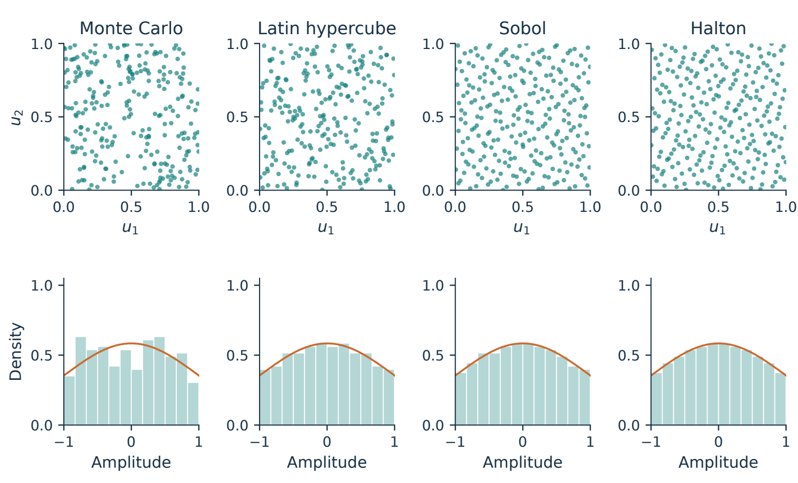
Figure 3 separates finite design coverage from the common inverse-distribution mapping. Comparisons record sample size, seed or scrambling settings, variable order, bounds, physical scale factors, and correlation assumptions. Estimation-error comparisons require appropriate repeated designs and uncertainty analysis; a smoother histogram is not sufficient evidence.
Interfaces amplify modeling mistakes during automation
A deformation boundary cannot stop abruptly
Moving a local region while the neighboring mesh or constraints remain fixed can concentrate deformation in a thin layer of elements. Obvious overlap may be absent, yet elements can become severely compressed and develop Jacobian or volume problems. A numerically small tolerance cannot replace a mesh-quality check. The relevant quantity is the deformation gradient relative to local mesh size and transition length.
Fixed interface constraints, transition regions, and post-deformation mesh checks are therefore part of the model definition. A valid baseline does not make all extreme samples valid. Extreme amplitudes and combinations are checked before scaling the batch.
Local manufacturing offsets differ from assembly pose
Figure 4 distinguishes two superficially similar operations. Moving only one terminal’s CORE while its substructure stays fixed is a local manufacturing-deviation choice and creates a nonconforming interface. Moving the entire male side relative to the female side is an initial assembly pose: male CORE and its substructure must move together.
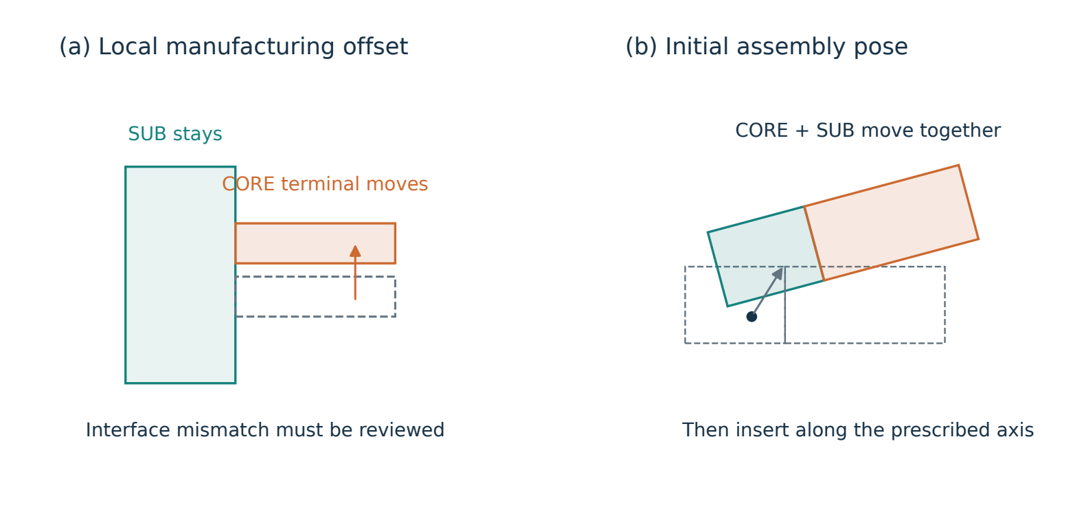
A tie constraint can connect a nonconforming interface. Increasing position tolerance changes which nodes or surfaces may enter that constraint; it is not a justification for repairing arbitrary geometric mismatch. Adjustment may undo an intended offset. Disabling adjustment instead requires checking actual tied coverage and its mechanical meaning. Abaqus documentation [2] explains these behaviors.
At minimum, code checks distances between corresponding labeled nodes, tolerance coverage, and whether the assembly input preserves the intended offset. The solver’s actual constraint establishment must still be verified. A large universal tolerance spanning nearby terminals makes automation more hazardous rather than more robust.
Split execution into recoverable stages
A stage matters more than one return code
Batch execution requires more than calling a solver in a loop. Each case is divided into recorded stages:
Prepare input Assemble Datacheck Solve Postprocess.
Passing datacheck does not mean a complete analysis has run. A successful outer process does not prove solver success. Logs, lock-file state, completion markers, and required steps and results in the ODB are checked together.
Each attempt has its own directory so old output cannot masquerade as a new result. Records identify inputs, selected tolerance row, substructure library, application release, CPU and memory settings, stage times, and failure locations. These records often carry more meaning than an isolated result CSV.
Concurrency, cores per job, and memory are separate controls
CPU cores per job differ from the number of concurrent cases. If each solve uses cores and up to heavy jobs run together, at least where is the active-job set and is a scheduling memory budget. A solver memory percentage is a configuration cap, not a measured peak or physical memory already reserved by the operating system. Preprocessing, postprocessing, mesh export, and filesystem caches also require headroom.
Python threads may coordinate external processes, while separate native solver processes perform the finite element work. Creating a large thread pool for every search path multiplies concurrency. A shared queue instead applies separate limits to mesh export, substructure generation, and full solves.
Recovery is not deleting a lock file
Interrupting a notebook kernel can leave external solvers running. Recovery must establish whether prior jobs are alive before resubmission. A state file or deletion of .lck alone is insufficient. Completed cases are reused; failures and unknown states require explicit retry choices.
Configuration changes need separate treatment. A scheduling-concurrency change can retain the same physical results after a safe stop. Changing friction, insertion endpoint, tolerances, model, or relevant code identity cannot silently mix new outputs into an old batch. Input hashes and frozen configuration make that distinction enforceable instead of relying on operator memory.
Define contact performance before ranking it
The metric concerns normal contact performance rather than treating a total reaction as the force in a specific contact pair. For pair , let be its total normal-contact-force vector. This implementation takes its global Y component: The output CFN2 is the second coordinate component of the normal-contact-force resultant. It is neither nodal contact pressure nor, in general, the vector’s magnitude. Changes in initial angle require checking that this global component still matches the engineering criterion. A component and a vector norm are not interchangeable.
At the specified final insertion displacement , define Here, is the number of required contact pairs and is the configured engineering threshold. A negative margin means at least one pair is below threshold. A nonnegative margin means every required pair reaches the threshold at the verified endpoint. Actual project thresholds, insertion endpoints, and dimensional calibration values are not disclosed.
Each case is ranked by its own minimum before minima are compared across cases. The weakest pair can change with tolerance or pose; a search cannot fix one pair in advance and ignore the rest. CSV outputs retain curves for all channels, endpoint values, and the weakest-pair identity so changes in rank can be inspected.
The endpoint must actually have been reached. The final step, step time, insertion displacement, and required channel count are checked. A low force from an interrupted solve cannot enter ordinary physical-failure ranking. Missing channels are not filled with zeros.
Search an operating boundary, not only a worst sample
Change the initial pose before insertion
An initially tilted insertion differs from applying a rotation after full insertion: their contact paths are different. For a fixed manufacturing-tolerance vector , the coordinate convention is where is the rotation center, the unit rotation axis, the initial angle, a global unit translation direction, and a signed offset. The prescribed insertion follows. Rotation and translation order is part of the model because they generally do not commute.
Existing local manufacturing offsets rotate with the entire male side. Its substructure and CORE move together, while the female stays fixed. Reference points, coupling control points, and interface nodes must be included in coordinate checks, not just the visible solid mesh.
Offset-only search: coarse scan, then refine crossings
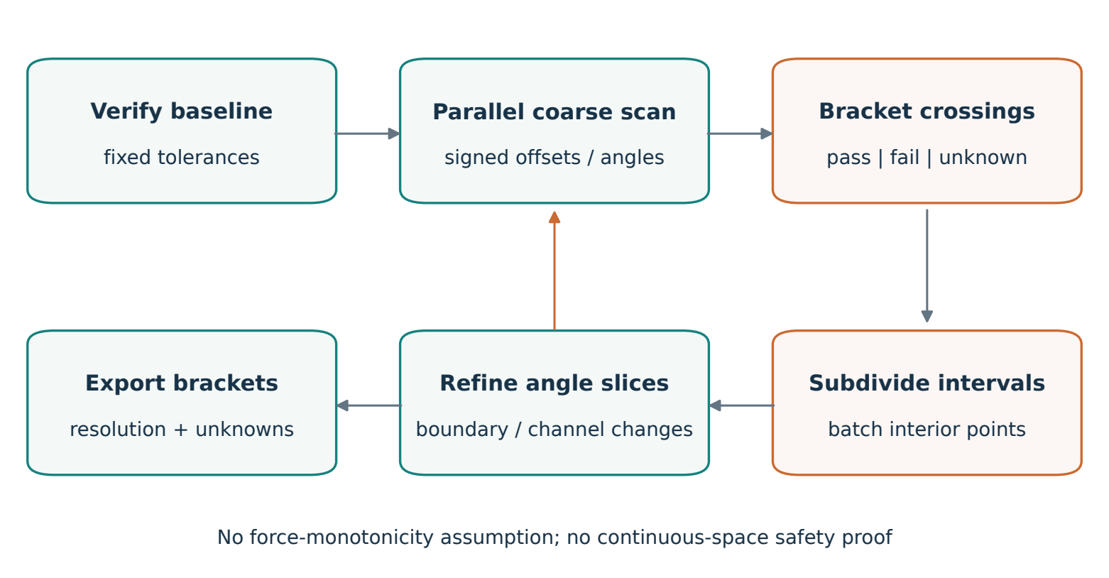
After a verified zero-pose baseline, positive and negative offsets are scanned in parallel within the configured range. Completed points are ordered by offset magnitude. Adjacent points whose values have opposite signs bracket a sampled crossing. Refinement can divide a bracket into parts and submit up to interior points together instead of evaluating only one bisection midpoint at a time.
The method does not assume that force decreases monotonically with offset. If a coarse scan passes, fails, and passes again, it retains multiple crossings and refines their intervals. The primary result is the first sampled failure boundary encountered from the origin, with all observed crossings retained.
Search stops when a discovered crossing bracket meets the offset resolution or a range limit, computation budget, or unresolved error is reached. The result is a pair of verified pass/fail points, not an interpolated exact limit. If failure is not found within the configured range, that absence is reported; the search bound is not relabeled as the actual mechanical limit.
Coupled offset and angle: one queue across slices
In a two-dimensional slice , selected initial angles each receive positive- and negative-offset searches. Slices share one queue, so other paths can progress while one awaits a solve. Intermediate angles are added when angular gaps are large or boundary location, weakest-pair identity, or slice status changes substantially.
Figure 5 illustrates this batched adaptive bracketing process. It is not reinforcement learning. A threshold-proximity curve such as can help visualize progress, but that auxiliary score does not replace the mechanical criterion or imply a learned policy or value function.
At a fixed angle, translating the entire assembly side leaves the substructure’s internal stiffness relationship unchanged. A verified library for that angle may therefore be reused with instance translation at the usage level [1]. The current implementation generates a male-side library once per distinct angle and shares a read-only cache across offsets. Cache provenance and artifact completeness must be checked; files left by a failed generation job do not make a usable library.
State what a boundary map does not cover
A slice of X translation and rotation about Y is not the full pose boundary with every translation and rotation varying simultaneously. The worst boundary for one fixed tolerance vector is not a reliability boundary for the random manufacturing population. Probability claims require a separate sampling design, coverage definition, and statistical uncertainty analysis over manufacturing variables and pose.
A finite coarse grid can miss a failure island narrower than its spacing. Two adjacent passing points do not prove that every intermediate point passes. Plots therefore retain pass/fail bracket bands, coarse-scan scale, refinement rules, and unknown regions rather than coloring everything beyond a smooth line as guaranteed safe. This is the conclusion supported by the algorithm’s actual coverage.
Acceptance checks for the complete system
| Layer | Questions to resolve |
|---|---|
| Geometry and interfaces | Is the baseline unchanged? Are coordinates, fixed regions, control points, and interfaces correct? |
| Physics and numerics | Are materials, contact, prepress, and insertion consistent? Do distortion or unintended ties affect results? |
| Execution and recovery | Did datacheck pass and solving complete? Could a retry duplicate a still-running job? |
| Postprocessing | Are pair identities and global components correct? Did final time and displacement reach their endpoints? |
| Search and interpretation | Do completed points support the brackets? Are unknowns, budget, resolution, and coverage recorded? |
Development checks can use known functions to test sampling, out-of-order parallel completion, bracket convergence, and recovery. Small artificial meshes test transformations and interfaces; real exported meshes test moved and fixed nodes. These checks establish software behavior, not a connector’s physical limit. Deployment still needs complete small-scale baseline, offset-only, and coupled offset–angle solves before expanding the search.
The implemented code connects sample generation through batch postprocessing and provides a parallel pose-search entry point with caching, budgets, and recovery state. The new whole-side-offset and coupled paths still require real-solver acceptance in a matching environment. No unverified critical angles, failure probabilities, or speedup factors are reported.
Build interpretability into automation
What makes simulation scalable is a sequence of explicit agreements: how regions and retained degrees of freedom are selected, how amplitude becomes dimensional change, which inputs remain fixed during comparison, what counts as completed solving, and which parameter subspace a boundary curve represents.
Substructures reduce repeated work. Recorded Tcl turns known GUI actions into parameterized operations. Bounded sampling makes probability assumptions reproducible. A shared queue and persistent state make batches manageable. Consistent contact metrics connect the samples to an interpretable boundary question. Every curve should lead back to its inputs, and every failure should have an explicit category. A smooth-looking plot alone is insufficient.
Reproducibility and public materials
Independent Python/Matplotlib scripts generate the figures, which are checked and exported through Tavotto and inserted as vector PDFs into the XeLaTeX text. Published sources contain only anonymized method descriptions and demonstration sampling; they do not read actual engineering files. The public website repository records the published source history.
References
Dassault Systèmes. Using Substructures. Abaqus documentation. https://docs.software.vt.edu/abaqusv2025/English/SIMACAEANLRefMap/simaanl-c-superelements.htm. Method reference; APIs must be checked against the installed runtime separately.
Dassault Systèmes. Mesh Tie Constraints. Abaqus documentation. https://docs.software.vt.edu/abaqusv2025/English/SIMACAECSTRefMap/simacst-c-tiedconstraint.htm.
McKay, M. D., Beckman, R. J., Conover, W. J. (1979). A Comparison of Three Methods for Selecting Values of Input Variables in the Analysis of Output from a Computer Code. Technometrics, 21(2), 239–245. https://doi.org/10.1080/00401706.1979.10489755.
Sobol’, I. M. (1967). On the distribution of points in a cube and the approximate evaluation of integrals. USSR Computational Mathematics and Mathematical Physics, 7(4), 86–112. https://doi.org/10.1016/0041-5553(67)90144-9.
Halton, J. H. (1960). On the efficiency of certain quasi-random sequences of points in evaluating multi-dimensional integrals. Numerische Mathematik, 2, 84–90. https://doi.org/10.1007/BF01386213.
SciPy. Quasi-Monte Carlo submodule: scipy.stats.qmc. https://docs.scipy.org/doc/scipy/reference/stats.qmc.html.
Tavotto. Technology: script, editable figure, replay and export. https://www.tavotto.com/technology/.
English PDF · Chinese PDF · Bilingual LaTeX and figure sources